
Are We There Yet?
Decision-making under extreme uncertainty in the COVID-19 pandemic
This post originally appeared on the CAIMS blog on May 15th, 2020.
As we’ve all come to know, flattening the curve is the process of reducing the number of infections and easing the burden on the health system during the COVID-19 pandemic. Protective measures, such as travel restrictions, social distancing, staying home and basic hygiene, have been implemented with success to flatten the curve. Comparisons across countries with different approaches, timelines and levels of government intervention indicate that slowing the spread of the disease is possible via these intervention strategies. In this post, we explore how we can provide the best scientifically-based evidence for such decisions.
There is no shortage of data for COVID-19. Indeed, global counts of confirmed cases and deaths are seemingly everywhere. We hear daily updates on the news and we see digital dashboards showcasing global maps and curves of cases, which have proliferated following the data dashboard popularized by the Johns Hopkins University team (find a non-exhaustive list of apps here, see a list of global and regional data interfaces here and here). How does one use this data to better understand underlying mechanisms of the disease?

Mathematical modelling
To do this we must move beyond graphing the curve and implement an epidemiological model. Epidemiological experts base their analysis on SEIR epidemic models. These models are deterministic differential equation models, which classify the population in susceptible, exposed, infected, and recovered sub-groups. A nice discussion of those models is given by Dan Coombs in an earlier blog post,and Alison Hill has provided a detailed implementation of the SEIR model with extensive documentation and references here.
The SEIR model is composed of compartments based on the progression of the disease. The parameters of the SEIR model describe the rate at which individuals move into different compartments, i.e. as susceptible individuals get exposed, or infected individuals recover or die. Clinical observations are used to determine some of these parameters, for example time to recovery, or duration of ICU admission. The recently released scenarios by the Government of Alberta are timely examples of such models in action for emergency preparedness and capacity building.
Unfortunately, the parameters concerning the infected individuals with less severe symptoms or without any symptoms are uncertain, and estimating the prevalence and incubation periods for these groups is more difficult. There is also variation among individuals depending upon pre-existing conditions, gender and age, which can result in biased estimates, particularly when testing selectively focuses on high risk groups.
Another consequence of individual variation is that the incubation periods vary drastically between infected individuals, some individuals being still infectious after the mandatory 14-day quarantine period. Focusing on a strict deterministic rule and ignoring the individual variations may lead to an incomplete understanding of the risk associated with such rare events.
Statistical modelling
As an alternative to previous approaches, we formulate a hierarchical statistical model to link observation to epidemiological mechanisms. Hierarchical models are statistical abstractions for situations when, for example, the true numbers of new infections are not directly observable. The deterministic SEIR model captures how the infections are changing over time. However, this model doesn’t describe how the true infections are related to the observed number of cases; this is where a hierarchical model can help. A hierarchical model provides the means to connect observed and latent processes, and to estimate model parameters and their associated uncertainties. This is important, as failure to account for observation error can lead to biased and misleading estimates of epidemic parameters.
Our hierarchical model requires detailed data on the daily number of new cases within small geographic areas. We chose Alberta as a test case because it is close to home and such data has been published by Alberta Health for 132 local geographical areas. Yet the same model can easily be applied to other jurisdictions as well. Now let Yi,t be the observed number of daily cases in area i on day t, and Ni,t be the true number of daily infections in area i on day t. Let Ni,t be a random variable that follows a Poisson distribution with rate λi,t, or in shorthand: (Ni,t | λi,t) ~ Poisson(λi,t).
The variable λi,t is also the expected number of true cases per unit time (days in our example) from a Poisson process. The rate takes positive values and can depend on covariates: log(λi,t) = Xi,tTβ, where X is a design matrix with the covariates as columns and β is the coefficient vector describing the relationship between the covariates and the rate parameter. The rate parameter can be a function of area specific demographic and census data, e.g. proportion of age classes, occupations, the size density of the population.
The rate can also depend on time varying effects, such as interventions, weather, or the true number of cases on previous days. These temporal dynamics can capture community transmission within areas with already positive cases. The proximity to such hotspots can introduce spatial dependence and travel-related infections into the model. For example, the number of infections in the neighbourhood two weeks ago might influence the true cases today. We would also expect interaction between temporal and spatial effects, e.g. neighbourhood effects would have been larger before travel restrictions.
How does this relate to the observed cases? We can describe the number of observed cases (Yi,t) as another Poisson distributed random variable: (Yi,t | Ni,t) ~ Poisson(αi,t Ni,t), where αi,t is the proportion of infected cases reported. The αi,t variable takes value between 0 and 1 and can be modelled on the logit scale as a function of covariates, such as changes in testing and reporting over time, the number of tests performed, demographic composition of the sample tested, lag time involved in testing. We can also use analogues to inform this part of the model, e.g. past influenza infection rates. If the spreading mechanism for influenza and COVID-19 is similar (infection rates might be different), then past flu spread should help us predict COVID spread.
Statistical models allow to estimate the model parameters (point estimates) and their associated uncertainty. This uncertainty in our cases is not normally distributed because of the exponential transformation used to link the covariates to the support for the random variable. This formulation inherently allows for longer tailed distributions and therefore provides a more realistic depiction of risk due to extremes from longer tailed distributions. Such characteristics of statistical modelling are most useful when making predictions about unobserved cases for during forecasting.
The ability to forecast the true number of cases for the different geographic areas with associated prediction error is the true advantage of the hierarchical state-space model outlined above. Understanding the spatio-temporal dynamics of the disease spread would help to inform future policy. For example, we can use the model to evaluate different scenarios based on the estimated number of actual cases rather than the observed number of cases.
Imagine, for example, that in a rural area with 0 current confirmed cases, there might already be an unknown number of infections, which number can be a function of nearby areas. This estimate can give early warnings for nearby hospitals to expect more patients and be an important tool in emergency preparedness. This prediction can be made more spatially accurate and precise by incorporating demographic data, like age, occupation, existing health conditions.
The model in action
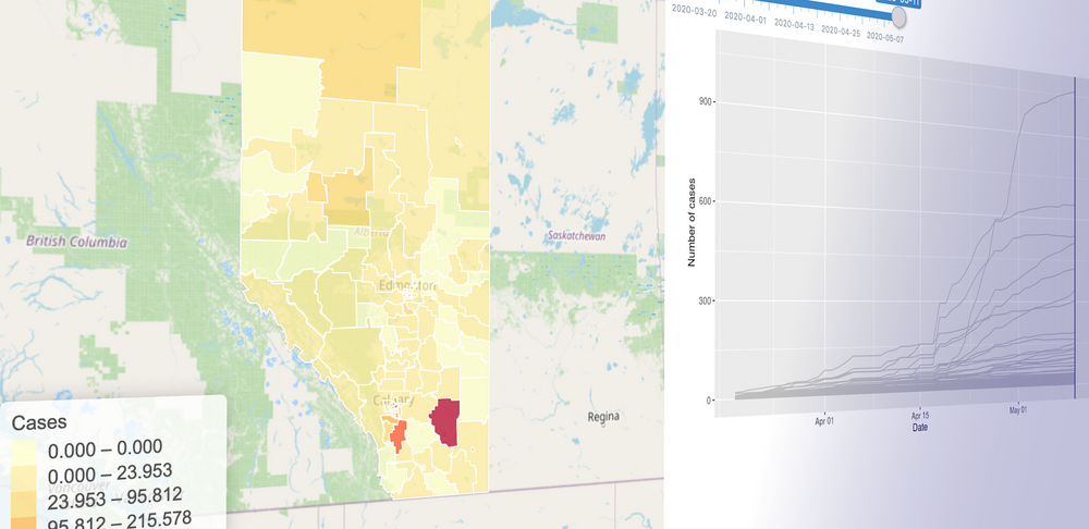
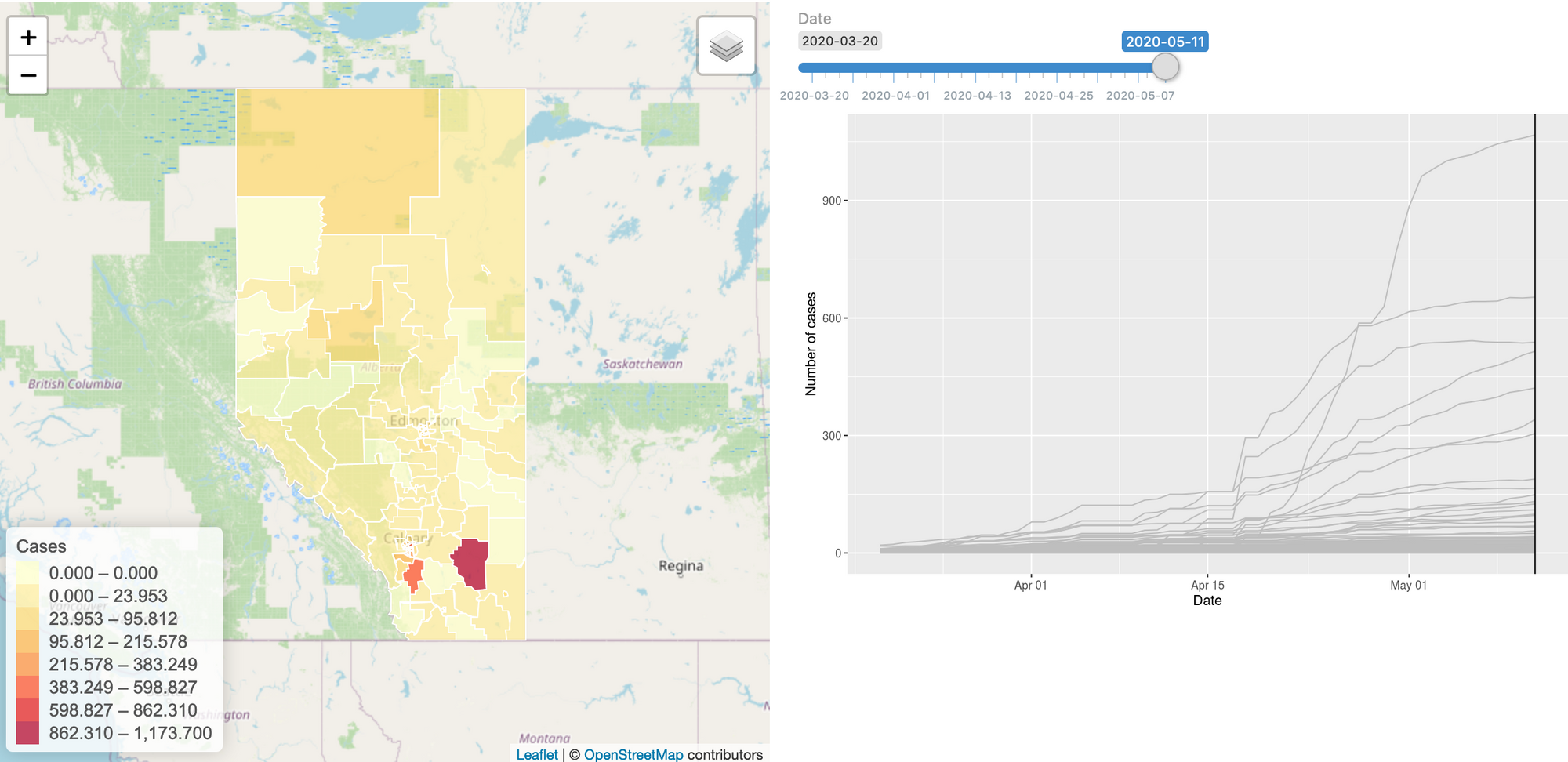
To build this model, we started gathering the data: we have daily case numbers from the 132 local areas in Alberta, the 2017 census data for population sizes, and the intervention dates by the Government of Alberta. We also include data from all countries around the world. We built a website (https://hub.analythium.io/covidapp/) where we collected relevant information about the COVID-19 pandemic.
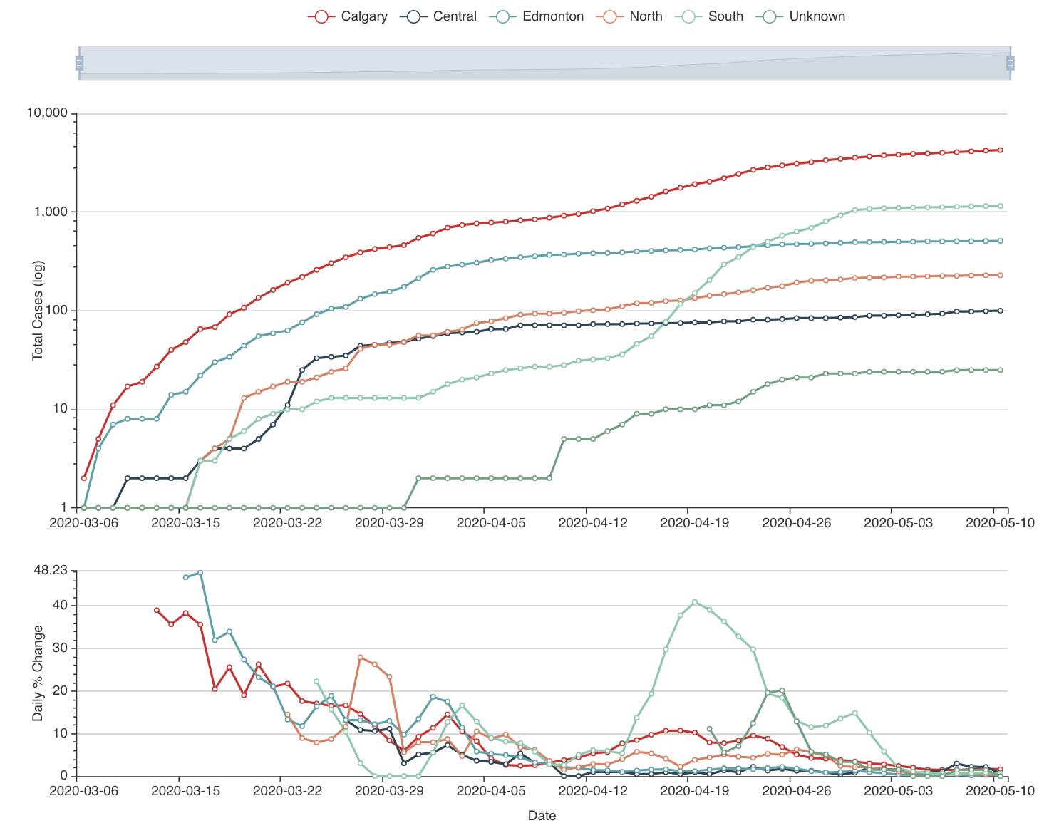
Users can look at different countries and see how the cumulative cases compare to each other (see linked video at the end of the post). Furthermore, they can also drill down to the Canadian data to explore cases between provinces and territories to compare daily cases, rates, and doubling times with interactive visualization. We also added the Alberta data by health regions and we are now working on even finer resolution data. We relied heavily upon the data by the Johns Hopkins team and the data provided by the Government of Alberta. Our scripts automatically update the data every day. The app in action can be seen at the end of this post.
The model can be refined by including key data, like demography, occupations, age distributions, etc. Other proxy information would also be very valuable, e.g. cell phone based average driving distances by regions. Another piece of information that would help to connect the true and observed cases is the reporting error for diseases with similar spreading mechanisms, i.e. influenza.
If you are interested in working with us to improve the website, help out with data collection, or modelling, please reach us at hello@analythium.io. We would love to take the hierarchical model to the next level to inform decision making with the best evidence during extreme uncertainty in the COVID-19 pandemic.


