Data most often comes in a tabular format where multiple columns contain variables (measurements) related to one another. For example, we can measure various chemical substances in air at a given sampling location (sample site) at a specific point in time. This sample and the corresponding measurements will then make up a row in our tabular data set. We can also measure air temperature, wind speed, etc. All these variables together are called multivariate data. This post describes some of the fundamental steps in 'exploratory data analysis' (EDA) using air quality data as an example.

We have introduced the Alberta Air Quality dataset in a previous post. There we explored spatial and temporal changes in the concentration of sulphur dioxide (SO2). We will use the same data set in this post, but this time using multiple variables.

Interactive Air Quality Data Visualization

Data exploration is the first step in the development of data analyticspipelines to facilitate better decision making. Analythium specializes inbuilding such analytics pipelines drawing upon domain expertise and usingpowerful statistical and machine learning techniques. In this post we explore a…

Analythium BlogPeter Solymos

The data set originated from the Alberta Air Data Warehouse. We included data from 19 sampling stations operated by the Wood Buffalo Environmental Association (WBEA). The number of variables varied between 10 and 19. Some stations have been operated since 1998, other since 2017. Our data set contained daily aggregates of the hourly measurements up till the end of 2019.

Variation in the data

Each variable can be characterized on its own. For example, we can look at the mean of SO2 from all the stations and years in determining that the mean was 39.9 ppb (daily maximum aggregate values). We can also determine that the values ranged between 0 (non-detect) and 113.1 ppb, this range is a particular measure of variation. Looking at variables in isolation and in combination (additive effect monitoring) is important for both environmental protection and human health. When looking at discrete variable concentrations one can compare a specific measurements against ambient air quality objectives (AAQO). Similarly, when looking at multiple variables one can compare the overall effects against the air quality health index (AQHI).

Covariation

When looking at two variables at a time we can assess their covariation. If the two variables tend to vary together, we say that they are correlated. For example, in our data set, ozone (O3) showed a negative correlation with relative air humidity (RH). The correlation is negative because when one variable increases, the other decreases. This tendency is visualized by the blue trend line in the following graph.

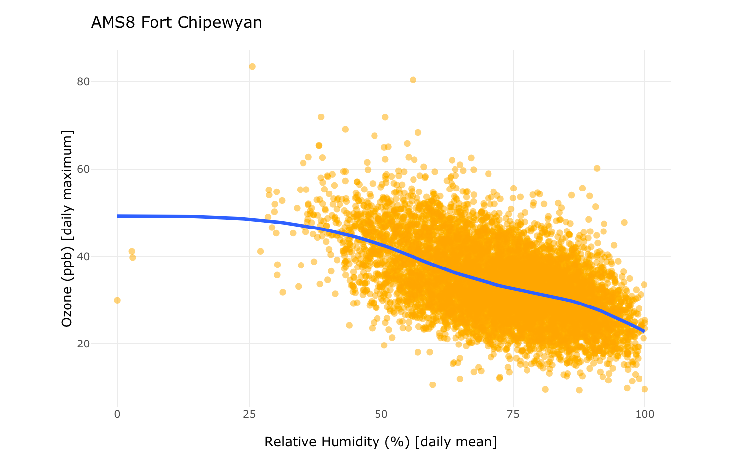
Such correlation is not sufficient for determining causation. Proving causation often requires mechanistic modelling and experimentation. But studying correlation can be an important step in the process of data exploration because exploratory data analysis can be used to generate hypotheses regarding causation.

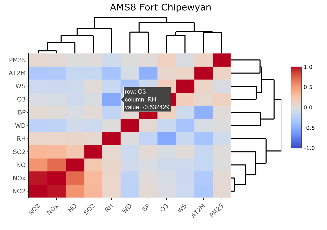
Heatmap

When we have more than 10 variables, a really useful way of determining the relationships between the variables is via a heatmap. A heatmap is a table like graph where rows and columns represent variables. The cells of this table-like graph represent the correlation based on the bivariate scatterplots, like the one above. For each pair of variables, we can calculate the correlation. If the correlation is negative, we colour the cell blue (see for O3 and RH). If the correlation is positive (when one increases, the other one increases too), we colour it red. The diagonal (red cells across) indicates perfect correlation when the row and the column is the same variable.

Interactive exploration

The interactive application below was built to explore the covariation among the variables. Follow the instructions at the top of the app and the Previous/Next buttons to see examples and explore the data. Variables can be logarithmically transformed to better reveal the differences among the lower values. Trend lines can be drawn based on the overall relationship, or year by year. Trend lines for the different years are coloured different shades of blue to help identify trends over time.

Get in touch

If you have similar data set and you would like expert advice on processing, transforming, analyzing your data or developing data integration pipelines or dashboards, schedule a free consultation to discuss your needs and how we can help. Sign up for our newsletter below to be in the know!